Adam is a lightweight optimizer for stochastic gradient problems that works fairly well. I never sat down to really understand it until now, but the design is delightfully simple with intuitive explanations!
Algorithm
The algorithm itself is quite simple. Here's the description from the paper itself:
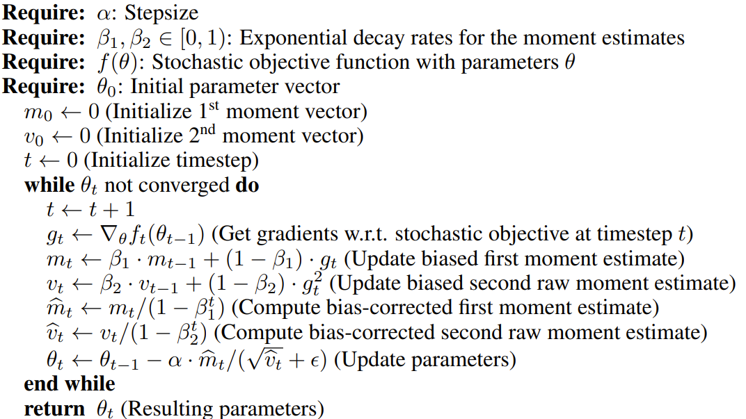
At a high level, there are only two moving pieces:
$m_t$- an EMA of the gradient$v_t$- an EMA of the square of the gradient
Because we initialize $m_0$ and $v_0$ to $0$, both will have a bias towards $0$ at the beginning of the process (as if all the earliest terms in the EMA were $0$). We fix this by scaling them up before using them in the parameter update:
Notice that as we see more samples ($t\rightarrow \infty$), the bias correction gets weaker: $\beta_{1,2}^t\rightarrow 0 \implies 1-\beta_{1,2}^t\rightarrow 1$.
Finally, the parameter update itself:
Intuition
This looks kinda strange, but there are two things going on here that make Adam better than regular SGD.
The first is momentum. If we wanted to write an update rule that only used momentum, we would write
Instead of updating the parameters with the current gradient, we update them with a moving average of the gradient. This has a few advantages:
- It averages out noise. When our objective function is stochastic (ex. we're computing it over mini-batches of a dataset instead of the whole thing), it's noisy, and any single gradient might be fairly off from the "true" gradient. A little bit of averaging does a lot to fix this.
- It helps avoid rapidly oscillating gradients. Imagine a narrow valley that has a sharp slope in one direction and a more gentle slope in another direction. If our start,
$\theta_0$isn't optimal in either direction, then the gradient along the sharp slope will shoot us back and forth across the valley, with the sign changing at each step. This oscillation isn't productive. But if we update$\theta_t$according to a moving average of the gradients, the updates to the sharp direction will cancel out, while the updates along the gentle direction will build up a true signal, pushing us in the direction of the optimum.
The second thing happening here is per-parameter learning rate equalizing. This is where the denominator $\sqrt{\hat{v}_t+\epsilon}$ comes in. Dividing our update by the EMA of the root mean square (RMS) of the gradient ensures that all parameters are being updated with around the same learning rate, $\alpha$. The intuition for this is that the gradient value for a parameter is not related to how far in parameter space we trust that gradient, and so we should largely decouple the magnitude from how much we update parameters.
Consider a parameter that has a very large gradient value. Once the RMS catches up, it will be equally large, and the update for this parameter will be normalized back to $\approx \alpha$. "But doesn't a larger gradient value mean we should update that parameter more?" No! A large gradient value means the loss landscape is changing rapidly as you move along that value. It does not mean that we trust that gradient information further out from $\theta_{t-1}$.
Consider a parameter that has a very small gradient value. The RMS for this will become small as well, which will normalize the update to this parameter also to $\approx \alpha$. This corresponds to a fairly flat region in parameter space. In order to move along flat regions in a reasonable amount of time, we need to make larger updates, hence scaling the update to this parameter up.